Get a Handle on AutoFill in Excel

AutoFill Handle

If you have used Microsoft Excel for any length of time, you have probably discovered the AutoFill handle — the tiny black square on the lower right-hand corner of a selected cell — to be one of its most useful tools. You can use the AutoFill handle to quickly drag a series into existence. You can drag days of the week, months of the year, or a numerical series — you can even create your own custom series.

Use AutoFill to enter the days of the week or months of the year

Even though Excel can’t sing, it knows the days of the week. You can begin a list by typing either the full day of the week or its 3-letter abbreviation in a blank cell. Then, position the mouse pointer above the AutoFill handle and drag the handle horizontally or vertically across adjacent cells. Dragging the handle down or to the right fills in the next item in the series, while dragging up or to the left fills in the previous item.

Similarly, Excel knows the months of the year. You can enter the month or its 3-letter abbreviation, then drag the AutoFill handle to fill in other months of the year.

AutoFill a numerical series

When it comes to automatically filling in a numerical series, you have a couple of options.

AutoFill Options button showing Fill Series option

First, if you select a cell containing a number and drag the AutoFill handle, Excel assumes you want to simply copy the value. When you release the mouse button, the AutoFill options button appears. Click the option for

Fill Series

to replace the multiple copies of the selected number with a series of numbers that increment (or decrement) by one.

Second, if you select two adjacent cells with distinct numerical values and drag the AutoFill handle, Excel fills the cells with a series which increments by the difference of the two values. In other words, if you selected one cell containing the number 1 and another cell containing the number 3 and then dragged with the AutoFill handle to the right, the resulting series would be 1, 3, 5, 7, etc. Each subsequent value would be 2 more than the last. In this way you can increment a series by twos, by threes, or even by twenty-sevens.

Customizing Excel’s AutoFill List

As we have seen, Excel knows days, months, and numbers — and that’s it. If you select a cell with any other “non-series” data and drag the AutoFill handle, Excel just copies those cells. However, you can create your own custom list — or lists — to “teach” Excel new series.

Let’s teach Excel the first ten ordinal numbers, first through tenth. In Excel 2003, click

Tools > Options > Custom Lists

. Then select

New List

and type each list entry, separating the values with commas. Finally, click

Add

, then

OK

.

Excel 2003 Custom List in Options dialog box
Note: In Excel 2007, click the Microsoft Office button, then click Excel Options. Click the Popular > Top options for working with Excel > Edit Custom Lists.

Now, you can AutoFill a series based on items in your custom list. And, you can even sort your data according to the order of items in your custom list.

AutoFill isn’t always a drag

You can extend a series in a column by double-clicking the AutoFill handle; Excel uses the column to the left as a guide.

Toggle the display of formulas on a sheet in Excel

When working in Excel, you may wish to see the formulas in use on your worksheet to help you track down an error, or to see which cells are dependent upon other cells.

To toggle the display of formulas on a sheet:

  1. In the Tools menu, click Options.

  2. On the View tab, in the Windows options area, check Formulas.

  3. Excel Options Dialog box Excel Options Dialog box
  4. Click OK.


Excel displays the formulas contained in cells on the active worksheet; it displays the underlying serial numbers for dates, and opens the Formula Auditing toolbar.

Excel spreadsheet with formulas displayed Excel spreadsheet with formulas displayed

Note: Alternatively, you can toggle the display of formulas in Excel by pressing CTRL + ` (grave accent).

Set up reliable data validation in Excel

You can use data validation to restrict the type of information allowed in a given cell (or cells). You can also specify a range of valid data for numerical, time or date values, and even text length. In addition, you can use data validation to limit data to a predefined list of acceptable items.

To set up data validation:


  1. Select the cells you wish to affect.

  2. Cells you wish to affect Cells you wish to affect
  3. In the Data menu, click Validation.

  4. The Data Validation dialog box appears.

    Data Validation dialog box Data Validation dialog box
  5. On the Settings tab, in the Allow box, click List.

  6. In the Source box, type the values, separated by commas, you want to allow.

  7. For example, try typing: blue, green, orange.
  8. Click OK.

  9. When you click on a cell, the drop-down arrow is available with the values you specified.

    Data Validation dropdown list Dropdown list

Note: In the Source box, you can use a formula or reference to a range of cells that contain your list values rather than explicitly typing those values in.

However, if you want to refer to a range of cells on a different worksheet in the same workbook, you need to define a named range, then refer to the named range in the Source box, =named_range.

Use the Lookup feature to find values in lists with vLookup in Excel

You can use VLOOKUP or HLOOKUP to find corresponding information in a list of data, either vertically (VLOOKUP) or horizontally (HLOOKUP).

The VLOOKUP function scans vertically down the leftmost column of data, looking for a match to the input you provide. Upon finding a match, VLOOKUP returns a value from the given row, corresponding to a column you specify.

Note: HLOOKUP functions similarly, but it scans horizontally across the first row of data and returns a value from a given column, with respect to a corresponding row number.

For example, if your data looks like the data in screenshot below, then this formula, =VLOOKUP("associate",A1:B4,2), would return 135:

VLookup Screenshot VLookup Screenshot

The three arguments required by VLOOKUP are Lookup Value, Table Array, and Column index. There is an optional fourth argument, Range Lookup.

  • Lookup Value: The data you want to find. This can be text (enclosed in quotes) or it can be a reference to another cell.

  • Table Array: A reference to a range of cells of at least 1 column of data. By default, the first column of data is used as the index to find the corresponding data for each row. Your data should be sorted in ascending order by the first column.

  • Column Index: The corresponding column that contains the data you want to return.

  • Range Lookup [optional]: A logical value, TRUE or FALSE. If this argument is omitted or TRUE the lookup returns the first closest match. If the argument is set to FALSE, lookup searches for an exact match.


Note: If you plan to copy your formula to use across more than one cell, you may wish to use absolute cell references for the table array so the addresses do not automatically adjust to a new range as the formula is copied. In our above example, the Table Array reference would become $A$1:$B$4.

Combining data from multiple cells with Concatenate in Excel

Excel gives you the ability to combine text from multiple cells into a single destination cell.

For example, if you have a cell that contains a first name and another cell that contains a last name, you can combine those cells together and also include arbitrary strings of characters such as a spaces (“ ”), or comma space (“, ”), or even whole words or phrases.

To combine text from multiple cells:


  1. Select the empty cell where you want the function to be stored.

  2. In the Insert menu, click Function.

  3. In the Category dropdown list, select Text.

  4. In the Function area, select Concatenate, then click Enter.

  5. Insert Function - Concatenate Insert Function - Concatenate
  6. Select Text1 in the Concatenate dialog box, then either click a cell on the sheet or type some text.

  7. Select Text2 in the Concatenate dialog box, then either click a cell on the sheet or type some text.

  8. Repeat steps 5 and 6 as necessary, then click OK.

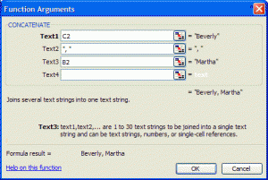
  9. Function Arguments Function Arguments

Note: In this example, the text elements for a last name, a comma followed by a space, and a first name are combined to make the text string “Beverly, Martha.”

You can use the “&” symbol to make your own concatenate string. This alternate formula would read =C2 & “, “ & B2.

Distributing data across columns with Text to Columns in Excel

In Excel, you can take a cell and split its text across columns in a number of ways. The easiest of these is to use the Text to Columns command under the Data menu in Excel.

For example, if you have a cell that contain both first and last names, you can use the Text to Columns command to split the data in each cell across multiple columns using a delimiter, a special character that indicates at what point data should be split. In this example, we will use a space as the delimiter.

To split text in a cell across columns:

  1. Select the cells you wish to affect.
  2. In the Data menu, click Text to Columns.
  3. In the Wizard, select Delimiter, then click Next.
  4. In the Delimiters area, check Space, then click Finish.
Before Text to Columns

Before Text to Columns

After Text to Columns

After Text to Columns